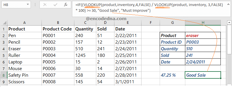
First, let us see a VLOOKUP() example.
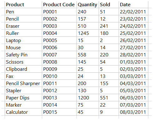
I have a table of data, a small inventory of stationary products (see the below image). A VLOOKUP is ideally used against a huge range of data, which might even spread to multiple sheets.
My inventory table looks like this.
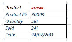
Now suppose, I want to find or look up the details of a particular product when I enter the name of the product in a cell. For example, if I enter eraser (the 3rd product in the above table), it should quickly find the product in the table and show other details like this.
The VLOOKUP() function takes four arguments in the form of, a "lookup value", "table array", "column index number" and finally the "matching criteria".

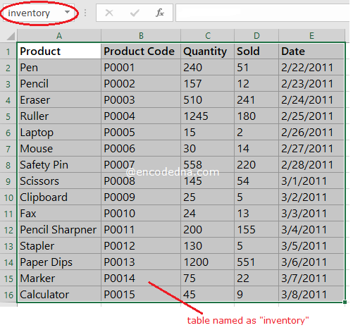
For the 1st two arguments, I'll create two named range.
For the 2nd argument: Create a named range on the table data and name it inventory. This is for the function’s 2nd argument (the table array). A named range will make the search easy and quick.
For the 1st argument: Create a named cell (a cell with a name), where the product name will be entered and name it product. This is for the lookup value (the function’s 1st argument).

Finally, I’ll add four formulas using the VLOOKUP() function in the subsequent rows where I’ll enter the product name.
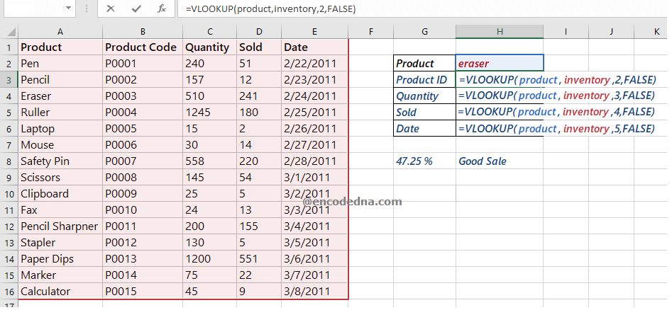
Its a very basic formula but useful.
See how I have used the two named range inside the function, followed by column index number (2, 3, 4 and 5). Now, when you enter a product name in cell H2 (for example pen), it will look-up the value pen in the table and get its other details and display the values in its respective cells.
Using VLOOKUP function with IF Statement
Well, we have added VLOOKUP in multiple cells. Now let's see how we can use the IF statement with VLOOKUP.
We often use the IF statement in an Excel formula when there’s a condition, and based on the condition we want to see our data.
In the above example, I want to check if the sale is a good sale or a bad sale, by calculating the sale percentage against the stock. Therefore, if the sale is greater than or equal to 30%, it’s a good sale.
Here’s the formula using VLOOKUP with IF statement.

The IF statement takes 3 arguments. The 1st argument is the logical test, where I am checking (with VLOOKUP) if the sale of the given product is greater than or equal to 30%. The 2nd and 3rd argument shows a result based on the logical test.
• I am also showing (although this is optional, I thought it’s worth sharing) the sale percentage of each product. The formula can be,
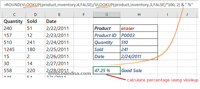
➡️ How to use IF statement in an Excel formula
The example that I have shared here, is a complete solution in itself, since I have used the VLOOKUP function multiple times, along with the IF statement, few important formulas, like calculating percentage and I have also shown how to create named range in Excel worksheet. I am sure will find the example useful.
Note: A VLOOKUP formula often throw an errors like #N/A when it fails to find a match. You can handle the errors and show a more meaningful message. Check this out.
More Excel Formulas
• A Simple formula to calculate a persons Age in Excel using the Year.
• How to use IF() and Nested IF() Functions in Excel
• Create Named Cells or Named Range in Excel and Use the Names in Formula or for Data Validation
• Excel formula to get Half-Yearly, Quarterly and Yearly date from a given Date
