Last updated: 31st July 2024
Use of date and time is common in Excel and we often add a column or two showing date in our worksheet. We use dates in our reports, day-to-day transactions and more. Here in this post, I am sharing a simple Excel formula to get half-yearly, quarterly and yearly date from a given date.
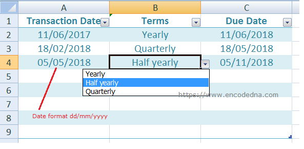
Let us assume, I have a column named transaction date (see the image above) in my worksheet. I want to show a due date (I’ll pick up my consignment on the due date or collect money from client, whatever), which can be "6 months" (or half-yearly) from the transaction date or the due date can be after 3 months (or quarterly) from the trans date.
I have 3 columns in Sheet1. A transaction date, followed by a dropdown list to select terms (like half-yearly, quarterly and yearly) and finally the column for "due date".
👉 If you don’t know how to add or remove a DropDown list in Excel, see this article.
Let's get on with the formulas. I am using a dd/mm/yyyy format for the dates in the examples here. Please check the date format in your Excel worksheet.
1) Formula to get "Yearly" date in Excel
=DATE(YEAR(A2), MONTH(A2) + 12, DAY(A2))
Copy and paste the formula in the 3rd column (under Due Date column).
📅 The DATE() function takes three parameters, that is, YEAR, MONTH and DAY. I am passing the Year, month and day from the 1st column (Transaction Date or A2) and adding "12" to the MONTH() function to get a date after 12 months.
Use the same formula to get half-yearly and quarterly dates. Simply add "6 and 3" to the MONTH.
2)Formula to get "Half-yearly" date in Excel
=DATE(YEAR(A2), MONTH(A2) + 6, DAY(A2))
3)Formula to get "Quarterly" date in Excel
=DATE(YEAR(A2), MONTH(A2) + 3, DAY(A2))
Simple isn’t it. Now let’s combine the formulas together using Nested IF statements, so we can automatically get the date based on our selection from the "Terms" dropdown list.
Date Formula using Nested IF
Copy this formula and paste it in the 3rd column (under Due Date). Click on the column again and drag it down to add the formula in multiple rows in the same column.
=IF(A2 <> "", DATE(YEAR(A2), MONTH(A2) + IF(B2="YEARLY", 12, IF(B2="HALF YEARLY", 6, IF(B2="QUARTERLY", 3, 1)) ), DAY(A2)), "")
Note: I am using a "dd/mm/yyyy" format for the dates in the examples here. Please check the date format in your Excel worksheet.
The first IF checks if the transaction date column is not empty. Next, I have added the DATE() function with multiple IF statements.

