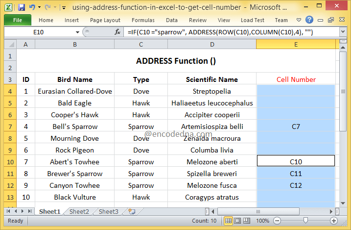
I said, Cell number of a specific text. See this image below.

I have a list of birds with name and type (also, the scientific name of each bird). Now, I want to get the cell numbers or the address of the cells that have a particular type of bird, let’s say the Sparrow or the Dove.
Here’s the formula!
=IF(C4 ="sparrow", ADDRESS(ROW(C4),COLUMN(C4),4), "")
In the above formula, I have used the ADDRESS() function inside the IF() function. You can use ADDRESS() inside other functions.
Hold the cell and drag the formula down to other rows.
The IF() function has three parameters. Now, here I am checking if a particular cell (like C4) has the value sparrow, if true then show the ADDRESS of the cell, if false then show nothing.
The ADDRESS() function has three parameters. Please see the complete syntax below. The first parameter is the row number; the second is the column number and third is the return type (4).
If the condition returns true, it would show the cell number in Column E.
Change the bird type inside the formula and see the result.
ADDRESS Function Syntax
ADDRESS (row_num, column_num, [abs_num], [a1], [sheet])
The first two parameters are important and required. The other three parameters are optional.
Note: You can simply type =ADDRESS( inside a cell in your worksheet to see the syntax.

row_num: It’s a numeric value in the form of a row number. This is required.
column_num: It’s a numeric value that specifies a column number to use. This is also required.
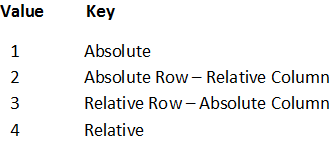
abs_num: The type of address the function will return. It’s a numeric value between 1 to 4. Although, I am using this parameter in my formula (above), this is an optional parameter.
abs stands for absolute. If you omit this value in the ADDRESS function, then the default return type is set to absolute or 1.
The four values and the return types:

Try this: In my formula above, I have used the value 4 and it retuned cells C7, C10 etc. Edit the number 4 with 1, 2 or 3 and see the result.
a1: The reference style, which is either A1 or R1C1. The values should be either TRUE or FALSE . Style A1 or TRUE is default.
sheet: The name of the worksheet you are using. If you omit it, the function will consider the default or current sheet your working.
Now, let’s fill all the parameters in the ADDRESS() function and see the result.
=ADDRESS(1,2,4,TRUE,"Sheet1")
Result:
Sheet1!B1
