Create Multiple Pie Charts in Excel using Worksheet Data and VBA

Click to enlarge the image!

Microsoft Chart Object for Excel provides all the necessary properties and methods to create charts in your Excel workbook, efficiently. You can create charts on your worksheet or create “separate” sheets with the charts. All you need is data.

👉 Do you know you can create multiple Line Charts automatically using a Macro? Check out this article.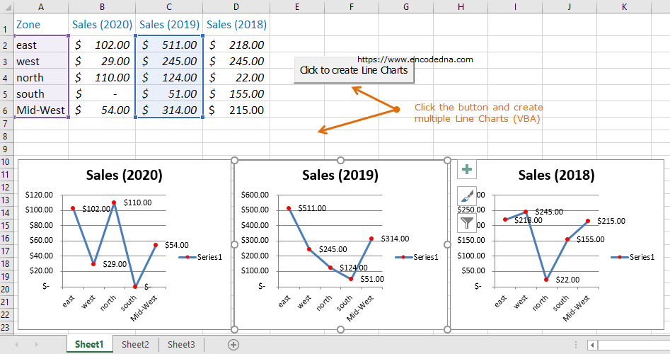

The data on my worksheet is similar to one I have used in my previous post. I just have few columns and rows. You can add more.

Next, add a button (an ActiveX Control) on sheet1.

The button’s click event will call the procedure createPieChart() to create and add multiple Pie charts, next to your worksheet data.

Option Explicit

Private Sub CommandButton1_Click()
    createPieChart
End Sub

Sub createPieChart()

    Dim src As Worksheet
    Set src = Worksheets("sheet1")      ' DATA ON SHEET1.
    
    Dim oChart As ChartObject           ' CREATE A CHART OBJECT.
    
    For Each oChart In src.ChartObjects
        ' DELETE PREVIOUS CHARTS (IF ANY). WE'LL CREATE NEW CHARTS FOR EVERY BUTTON CLICK.
        oChart.Delete
    Next
    
    ' AN ARRAY OF COLUMNS WITH DATA FOR THE CHARTS.
    Dim aRng() As String
    ReDim aRng(1 To 5)
    
    aRng(1) = "B2"
    aRng(2) = "C2"
    aRng(3) = "D2"
    aRng(4) = "E2"

    Dim pieChart As New Chart
    Dim oSeries As Series		' THE SERIES OBJECT REPRESENTS A SERIES IN A CHART.
    
    Dim i As Integer
    Dim ileft  As Integer
    ileft = 10          ' THE INITIAL LOCATION.
    
    For i = LBound(aRng) To UBound(aRng) - 1
        
        ' CREATE THE CHART.
        Set pieChart = src.ChartObjects.Add(Width:=200, Height:=200, _
            Top:=170, left:=ileft).Chart
        
        With pieChart
            .ChartType = xlPie     		' CHOOSE THE TYPE OF CHART.
            .HasTitle = True
            
            ' USE COLUMN NAMES FOR CHART TITLE.
            .ChartTitle.Text = src.UsedRange.Rows.Cells(1, i + 1)
        
            Set oSeries = .SeriesCollection.NewSeries		' NEW SERIES FOR A NEW CHART.
            With oSeries
                .XValues = src.Range(src.Range("A2"), src.Range("A2").End(xlDown))	
                .Values = src.Range(src.Range(aRng(i)), src.Range(aRng(i)).End(xlDown))
            End With
            
            ' ADD DATA LABELS TO EACH SERIES.
            .SeriesCollection(1).HasDataLabels = True
        End With
        
        ' SET NEW LOCATION FOR THE NEW CHART (CALCULATED BASED OF CHART WIDTH).
        ileft = ileft + 200
    Next i
End Sub

Now, just click the button and it will automatically add Multiple Pie Charts below the data (on the same sheet), along with Data Labels over each slice of the chart.

In the above code, first I am getting the data source for my Pie charts.

Dim src As Worksheet
Set src = Worksheets("sheet1")

Next, I’ve created a chart object to check if any chart exists on my worksheet. Every time you click the button, it will create a new instance of the charts and add it. Therefore, you need to delete the previous instance of the charts. Else, you will create multiple charts, one over the other.

Therefore, delete previous instances of charts.

Dim oChart As ChartObject

For Each oChart In src.ChartObjects
    oChart.Delete
Next

I’ll now create an array for a range of data. See the above image; I have data (units sold) in columns B to E. Each column has rows of data, which will provide the values to each new series for a new chart.

Dim aRng() As String
ReDim aRng(1 To 5)

Finally, (inside the For loop) I am adding a new chart using different coordinates.

Set pieChart = src.ChartObjects.Add(Width:=200, Height:=200, Top:=170, left:=ileft).Chart

The add() method takes four parameter, for the Pie location and its size (that is width and height). Since, I am placing the Pie charts horizontally, one after the other, the location left: is set as dynamic.

I am initializing the Series object with SeriesCollection. Every column of data on my worksheet is called a series. Therefore, I need a new series for my column of data.

Set oSeries = .SeriesCollection.NewSeries

Here, I am using two properties of the Series object.

1) XValues, to set an array of x values for my Pie chart series. The XValues property can be a array of data or a range in your worksheet. In my example here, it’s a range. The range is a static A2 and all the rows in this range (the month). This remains same for the all the charts.

2) Property Values to set a collection of all the values in the series. The value for this property can be a range on a worksheet or an array. For the example, I have set a dynamic range, starting for B2 to E2.

.Values = src.Range(src.Range(aRng(i)), src.Range(aRng(i)).End(xlDown))

I have also added DataLabels on each Pie Slice, as this will make the charts easier to understand.

.SeriesCollection(1).HasDataLabels = True

Note: Each Pie chart on your worksheet is Movable. That is, you can drag the charts and move it to a new location, anywhere on your worksheet or simply copy and paste the chart in another sheet.

You can also create Line Charts in Excel using a simple Macro.

← PreviousNext →