It saves time. I’ll tell you how I did this.
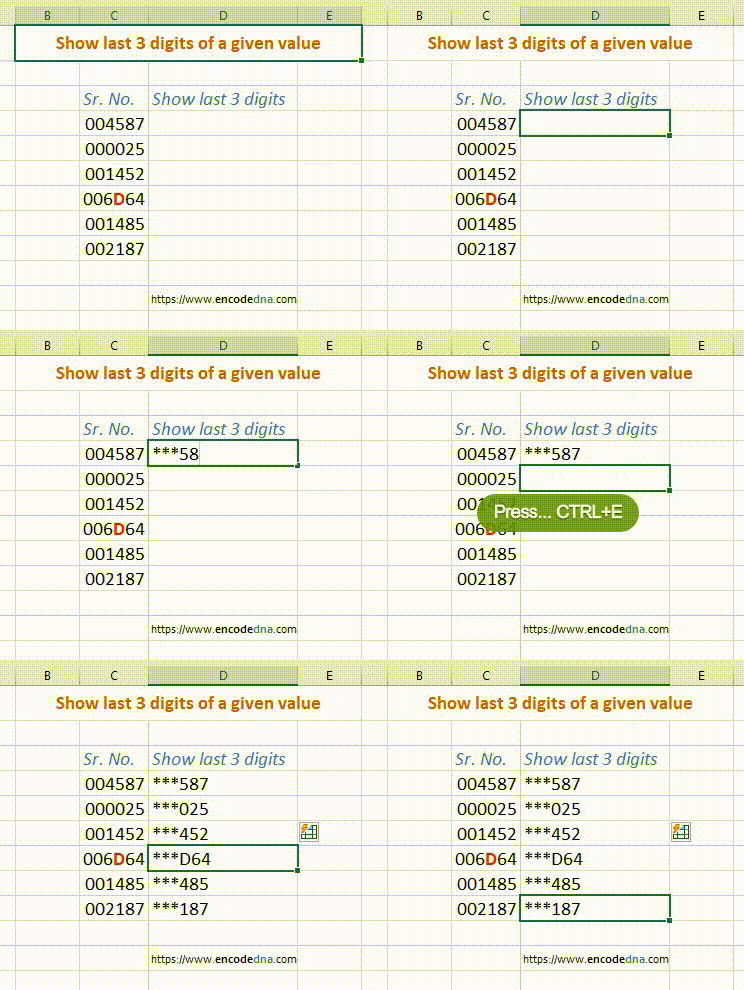
I am using a feature called Flash Fill in Excel. The first column has a list a value prefixed with two zeros. I’ll the mask the "first" three values, and show only the "last" three values in the next column.
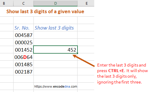
I selected the first value (cell D4) and typed three "*" (or asterix symbox) followed the last three digits in the next column. Then I shifted focus to the next row of the 2nd column (D5) and pressed CTRL+E keys and Excel "automatically" filled the remaining cells with values by sensing a pattern.
Note: You can set focus anywhere between the D4 and D9 cells, type a pattern (any pattern) and press CTRL+E.

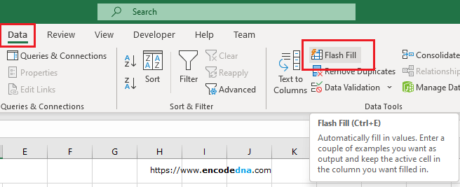
The shortcut key CTRL+E is for Flash Fill option. You can find this option inside Data Tools section in Excel.
In your Excel worksheet, select Data from the top menu and find Flash Fill option under Data Tools section (or group).

Remember, any changes you make to the values in the "first" column (the source), will not be be reflected in the "second" column (the result). You will have to apply flash fill again, manually.
