Excel IMAGE function Syntax
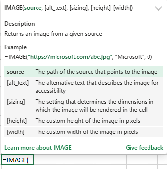
IMAGE(source, alt_text, sizing, height, width)

The IMAGE() function takes five parameters (or arguments). The function inserts an image using a URL.
The supported image formats are… png, jpg, jpeg, gif, ico and tif.
Note: Currently, the IMAGE() function is available only to users who have access to Microsoft 365 or Excel for the Web.
Well, if you do not have Microsoft 365 account, don't worry, you can still insert an image in your Excel worksheet by simply dragging and dropping the image anywhere on the sheet. You can place it or resize it according to you requirement. However, the image remains floating.
Now, let’s get back to the new IMAGE() function.
Like I said, the function takes five arguments.
1) source – The source of the image or the URL of the image. This is required.
2) alt_text – You can use this option to provide the image with a name or a description. This is optional.
3) sizing – This is optional. Use this option to set the dimension of the image. The values are,
0 – (default). It will fit the image in the cell using aspect ratio.
1 – Fill the cell with the image. It will ignore aspect ratio.
2 – Show the image as it is, that is, the original size of the image.
3 – use this value to set the image height and width.
4) height – You can assign a height (in pixel) to the image using this option. This is optional.
5) width – You can assign a width (in pixel) to the image. This is optional.
Add Image in a cell in Excel using a Formula
If you can access Microsoft 365, sign in to it and open Excel.
Choose a cell and write the IMAGE() function like any other function. For example,
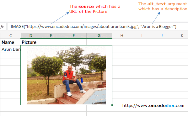
=IMAGE("https://www.encodedna.com/images/about-arunbanik.jpg", "Arun Banik", 1)Press the Enter key once you have finished writing the formula.

That’s it. Its that simple.
Here’s some important tip. When you first write the formula using the IMAGE function, it will adjust the image inside the cell. The image will not even be visible properly. That’s the default behavior.
Now, if you see the above image, where I have added my picture in Microsoft 365 Excel worksheet, the picture looks big enough and its clearly visible. How? I have used two options, Wrap Text and Merge & Center, after adding the picture.
The formula also has alt_text option (the 2nd argument), where I have described the picture with a small description.
Adding dynamic arguments to IMAGE function
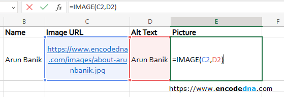
You can make this a little more dynamic by providing arguments to the IMAGE() function with values extracted from different cells.

This way you can create a table or list of products or places with images.
Common Mistakes with the IMAGE Function
Here are some of the most common mistakes users make when using the Excel IMAGE function and how to avoid them.
1. Using Unsupported Image Formats
Excel only supports specific formats: JPG, JPEG, PNG, GIF, BMP, TIFF, ICO, and WEBP (but WEBP isn't supported on Excel for Web or Android). Therefore, stick to widely support image formats like "JPG" or "PNG".
2. Using HTTP Instead of HTTPS
The source URL must use the https protocol. http links won't work. Always verify that your image URL starts with https://.
3. Quoting the URL Incorrectly
Make sure the "URL" is always enclosed in double quotes (" "). Therefore, use either "https://www.encodedna.com/images/about-arunbanik.jpg" or a cell reference like A1 if the URL is stored there.
4. Skipping the Sizing Parameter
Omitting the sizing argument can result in tiny or poorly scaled images. Always, use 1 to fill the cell or 3 for custom dimensions.
5. Incorrect Custom Dimensions
When using sizing = 3, failing to specify both height and width can cause errors or distorted images. Always provide both dimensions when using custom sizing. For example:
=IMAGE("https://www.encodedna.com/images/about-arunbanik.jpg", "Arun Banik", 3, 100, 100)6. Exceeding URL Length Limit
URLs longer than 255 characters may break the formula. Store the URL in a cell and reference it like this:
=IMAGE(A1)
