
To overcome these limitations, Microsoft introduced the XLOOKUP() function.
The XLOOKUP() function is a new alternative to VLOOKUP() that makes searching and retrieving data easier, more flexible, and more efficient.
In this tutorial, you will learn how to use the XLOOKUP function in Excel with simple, practical examples.
What is the XLOOKUP() Function?
The XLOOKUP() function searches for a specific value in a range or array and returns the corresponding value from another range or array.
Unlike VLOOKUP, XLOOKUP can search in both directions and performs an exact match by default.
Syntax
=XLOOKUP(lookup_value, lookup_array, return_array, [if_not_found], [match_mode], [search_mode])
- lookup_value: The value you want to find.
- lookup_array: The range where Excel searches for the value.
- return_array: The range containing the result to return.
- if_not_found: Optional value to display if no match is found.
- match_mode: Defines the type of matching.
- search_mode: Defines the search direction.
Example 1:
Here's a basic XLOOKUP Formula. Now suppose, you have an employee table with some data in it.
| Employee ID | Employee Name | Department |
|---|---|---|
| 101 | Rahul | Sales |
| 102 | Priya | HR |
| 103 | Amit | IT |
| 104 | Neha | Finance |
| 105 | Rohit | Marketing |
You want to find the department of employee ID 103. The formula will be,
=XLOOKUP(103,A2:A6,C2:C6)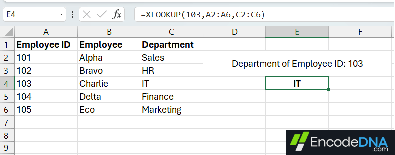
The parameters:
103 is the lookup value.
A2:A6 is the lookup array.
C2:C6 is the return array.
Example 2:
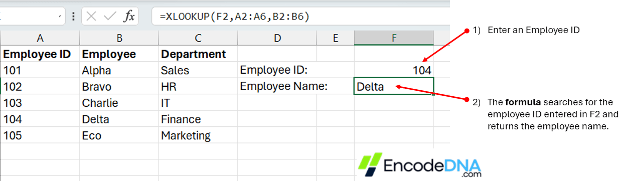
In the 2nd example, we'll use XLOOKUP with a cell reference. So, instead of entering a fixed lookup value, you can use a cell reference. You do have to hardcode the value.
Suppose cell F2 contains employee ID 104. The formula will be,
=XLOOKUP(F2,A2:A6,B2:B6)This formula searches for the employee ID entered in F2 and returns the employee name. The advantage is that you can change the employee ID in F2 without modifying the formula.
Example 3: XLOOKUP with a Custom Not Found Message
One useful feature of XLOOKUP is that it allows you to display a custom message when a lookup value does not exist.
=XLOOKUP(106,A2:A6,B2:B6,"Employee Not Found")This formula is useful when working with large datasets because it provides a meaningful message instead of an error.
Example 4:
You can use XLOOKUP to Search values from Right to Left.
One major limitation of VLOOKUP is that it cannot easily return values from columns located to the left of the lookup column. Suppose you table looks like this.
| Employee Name | Employee ID | Salary |
|---|---|---|
| Alpha | 101 | 25000 |
| Bravo | 102 | 30000 |
| Charlie | 103 | 35000 |
| Delta | 104 | 40000 |
You want to find the employee name using employee ID 103.
=XLOOKUP(103,B2:B5,A2:A5)The result will be: Charlie
Unlike VLOOKUP, XLOOKUP can search in one column and return a result from a column on its left.
Example 5:
Interestingly, you can use XLOOKUP to find approximate matches.
For example, you have "commission" table and you want to calculate the commission rate of ₹25,000. The formual will be,
=XLOOKUP(25000,A2:A5,B2:B5,, -1)
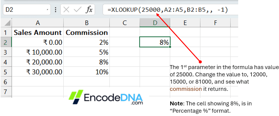
The match mode "-1" finds an exact match or the next smaller value. 👉 One This example assumes the sales amount column is sorted in ascending order.
Conclusion
The XLOOKUP() function is a powerful alternative to VLOOKUP() in Microsoft Excel. It offers greater flexibility, simpler formulas, and additional search capabilities.
If you regularly work with employee records, sales reports, product lists, or financial data, learning XLOOKUP can make your Excel work faster and easier.
Here's a VLOOKUP example. This will help you understand the function better.
More Excel Formulas
• A Simple formula to calculate a persons Age in Excel using the Year.
• How to use IF() and Nested IF() Functions in Excel
• Create Named Cells or Named Range in Excel and Use the Names in Formula or for Data Validation
• Excel formula to get Half-Yearly, Quarterly and Yearly date from a given Date